Tutorial with test dataset
In this tutorial we will show how CDCs CLI can be used on an example dataset of pumpkins to extract the pumpkins in the orthomosaic.
The example dataset can be downloaded from Zenodo on this link: https://zenodo.org/record/8254412.
The example dataset is from a pumpkin field, where the orange pumpkins can be seen on a gray background. save the example dataset in an easy to reach location on your computer, for this tutorial we will placed it in the following directory: /home/cdc/example_dataset.
The dataset consist of the following files:
an orthomosaic from a pumpkin field with orange pumpkins on a brown / green field 20190920_pumpkins_field_101_and_109-cropped.tif
a crop of the orthomosaic crop_from_orthomosaic.tif
an annotated copy of the cropped orthomosaic crop_from_orthomosaic_annotated.tif
To learn the color distribution, the information from the ccrop_from_orthomosaic.tif file is combined with the annotations in the crop_from_orthomosaic_annotated.tif file.
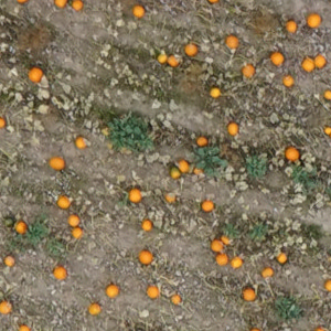
crop_from_orthomosaic.tif
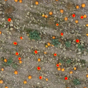
crop_from_orthomosaic_annotated.tif
If CDC is not already installed, see installation.
With CDC installed the CLI can be run with:
python -m CDC
or if the installation have added CDC to the path it can be invoked simply with:
CDC
From here on out we will assume CDC is in the path, but if that is not the case for you replace CDC in the following with python -m CDC.
To create a color model from the crop_from_orthomosaic.tif and the crop_from_orthomosaic_annotated.tif files and apply it on the orthomosaic 20190920_pumpkins_field_101_and_109-cropped.tif to calculate the color distance, use the following command in the dataset folder e.g. /home/cdc/example_dataset:
CDC 20190920_pumpkins_field_101_and_109-cropped.tif \
    crop_from_orthomosaic.tif \
    crop_from_orthomosaic_annotated.tif \
    --save_ref_pixels
This will take a little time but a progress bar will be shown.
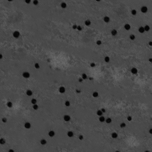
The output is new georeferenced orthomosaic with the calculated color distances to the reference color as grayscale. Here is a small part of the orthomosaic shown, right below is the same area in the input orthomosaic.
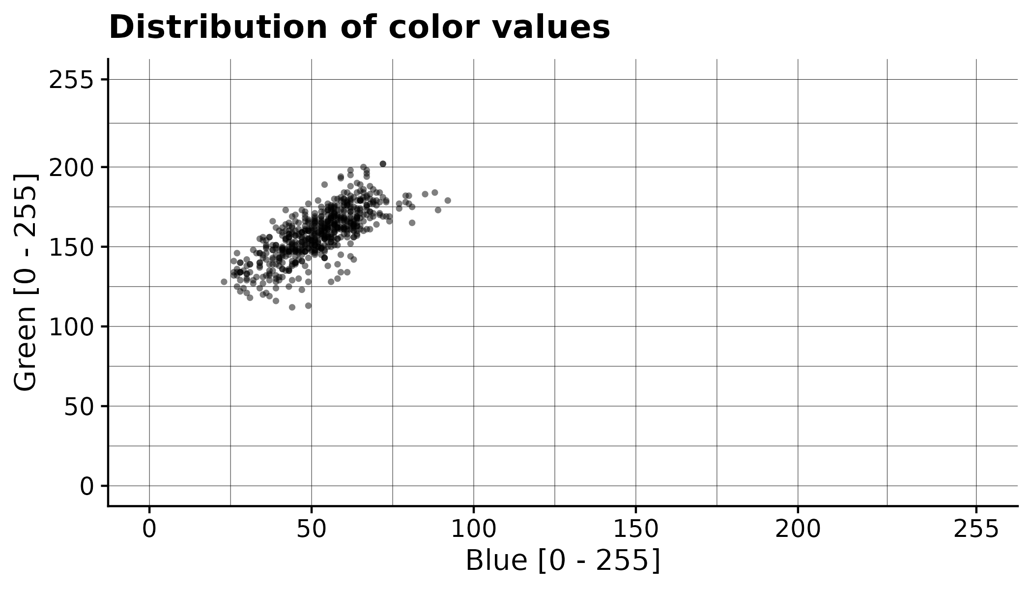
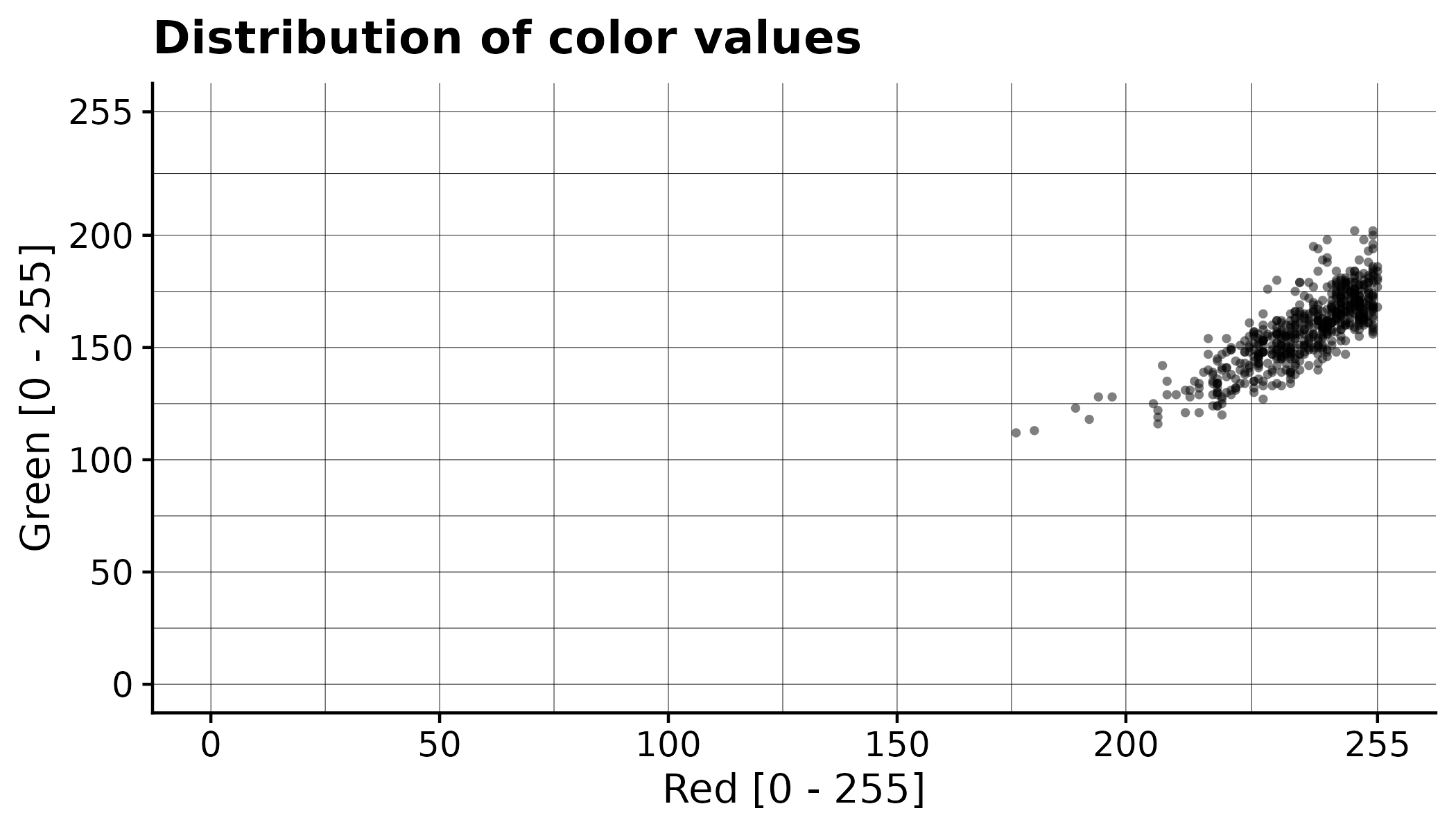
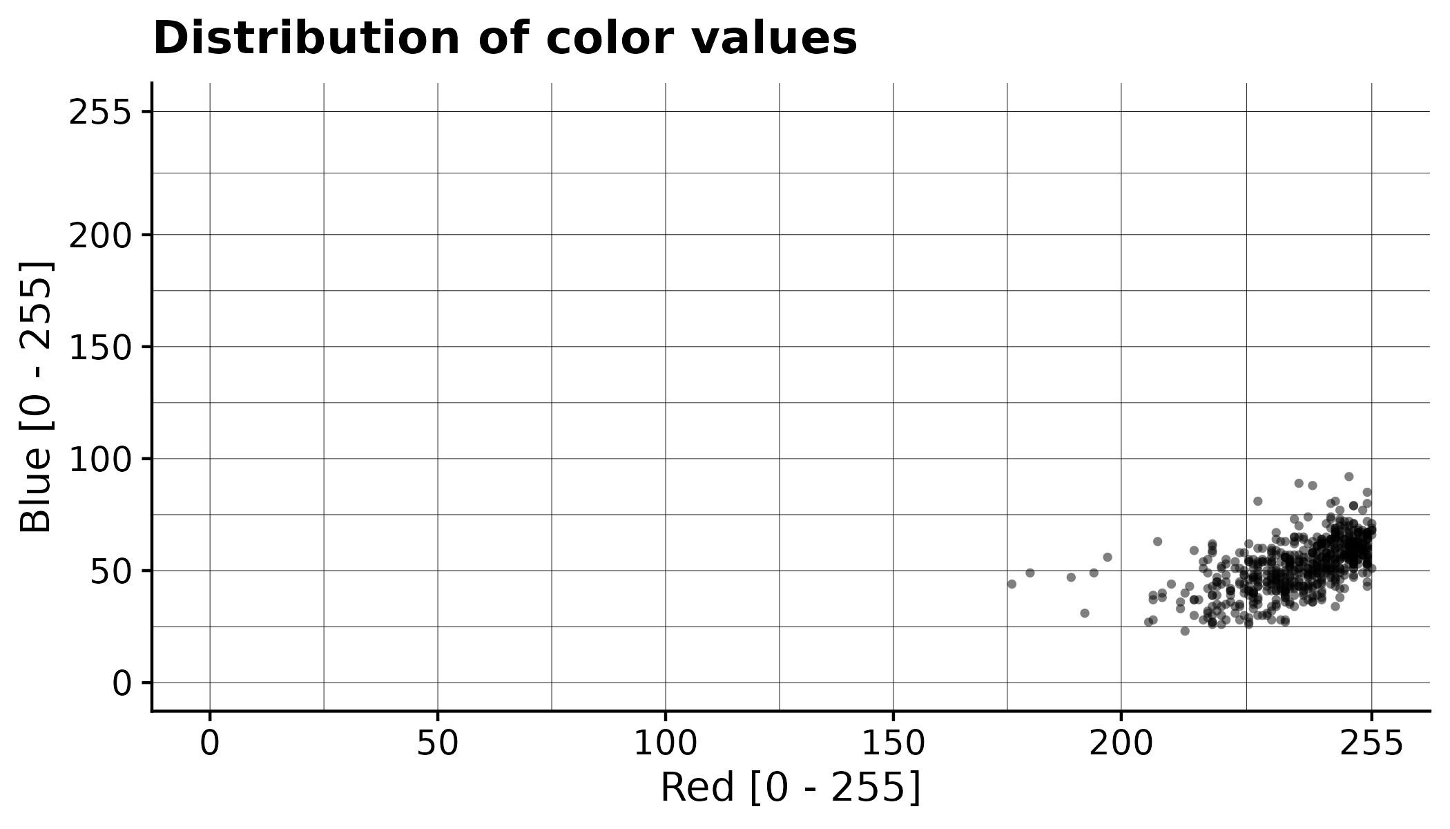
In addition to generating the processed orthomosaic, the CDC also have exported a file pixel_values/selected.csv that contains all the color values of the annotated pixels. This can be used to gain a better understanding of the segmentation process. Each row corresponds to the color value of one pixel.
r |
g |
b |
|---|---|---|
214 |
128 |
23 |
223 |
131 |
35 |
220 |
130 |
39 |
220 |
134 |
27 |
… |
… |
… |
Here the values from the example have been plotted:
If you would like to know more about how the algorithm for calculating the distances work see Calculate distances to reference color